Hello everyone,
I’d like to share a little experimental hike I enjoyed in Collatz land last week.
Preamble (known stuff)
Consider the parity vector [1,1,0,0,0] which is support to the rational cycle \frac{5}{23}, \frac{19}{23}, \frac{40}{23}, \frac{20}{23}, \frac{10}{23} :
>>> import coreli
>>> pv = coreli.ParityVector([1,1,0,0,0])
>>> pv.cyclic_rational()
5/23
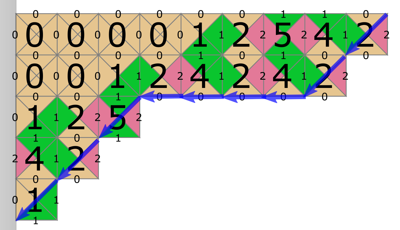
In terms of tilings, this parity vector corresponds to the following valued path:
[(↙,4), (↙,4), (←,0), (←,0), (←,0)]
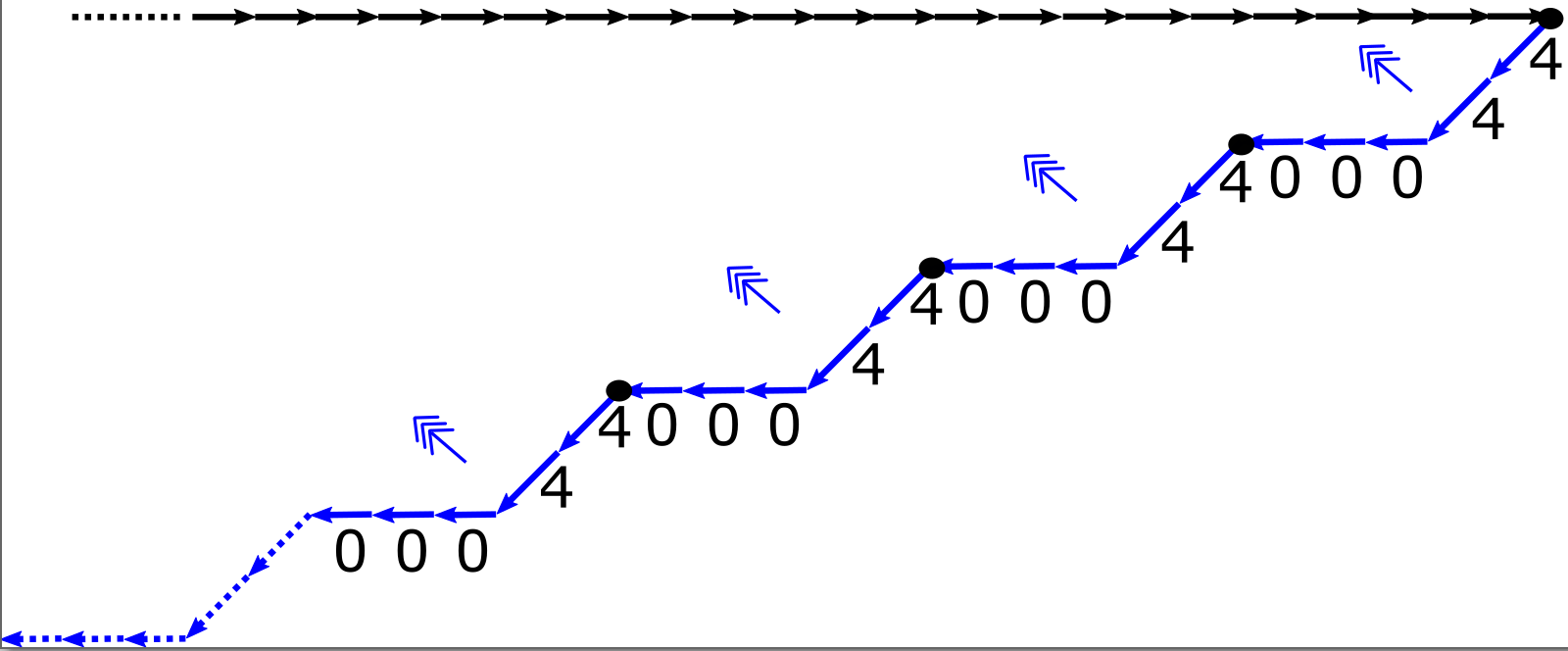
A valued path is a sequence of valued arrows.
A valued arrow is a tuple (arrow, value) with arrow in {←, →, ↑, ↓, ↖,↘, ↙, ↗} and value in of {0, 1} for horizontal arrows, {0, 1, 2} for vertical arrows, and in {0,1,2,3,4,5} for diagonal arrows.
Each valued arrow computes a function (see Figure 1.9) , e.g. the function computed by (←,0) is x \mapsto \frac{x}{2} and the function computed by (↙,4) is x \mapsto \frac{3x+1}{2}, sounds familiar? The function computed by a valued path is the composition of the functions computed by the arrows (Definition 1.9).
You van think of valued path as mixed bases representations.
Parity vectors are transformed to valued path in a trivial way:
- entries 0 of the parity vector are mapped to
(←,0) - entries 1 of the parity vector are mapped to
(↙,4)
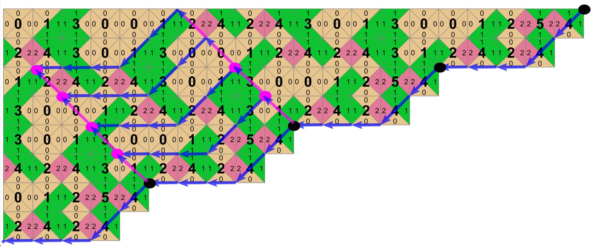
Then, if you lay out infinitely many copies of the valued path in space:
An you start tiling with the 6 Collatz tiles (you place tile 4 on each (↙,4) and south edge 0 on each (←,0), which is enough to uniquely tile the region top-left of the path because the tiles are deterministic in the top-left direction), you will see appear, 2-adic, 3-adic and 6-adic representations of the rationals of the cycle, here, \frac{5}{23}, \frac{19}{23}, \frac{40}{23}, \frac{20}{23}, \frac{10}{23} :
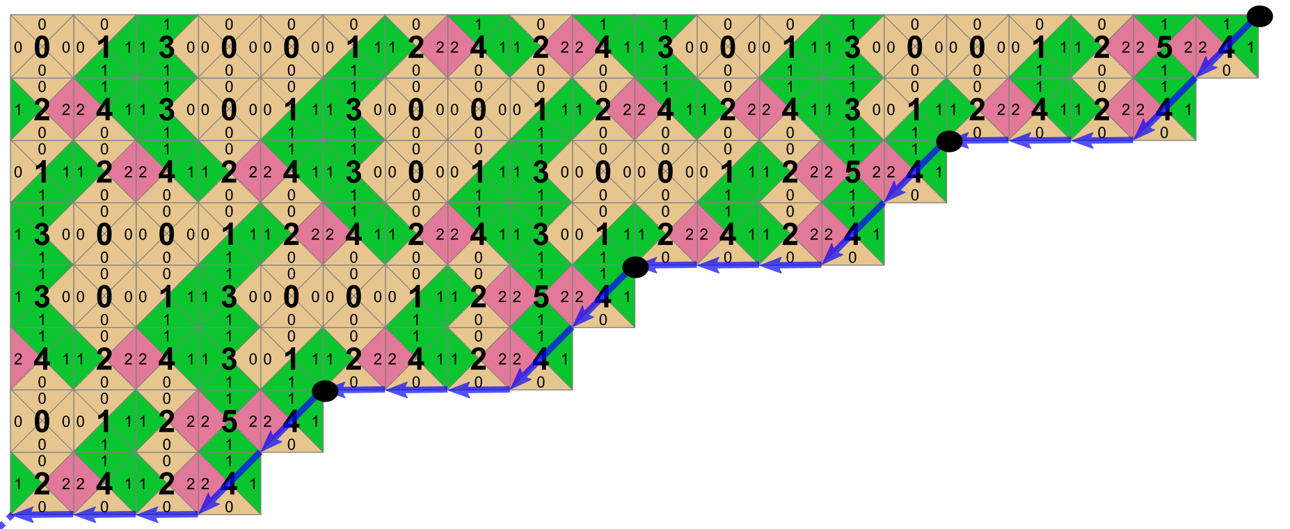
For instance, each line ending in a black dot reads (01100100001)* 1, which although might not be obvious at first sight, is the 2-adic expansion of \frac{5}{23} ![]()
>>> Z2 = coreli.Padic(2)
>>> Z2.from_rational(sympy.Rational(5,23)).rational_periodic_representation()
'(01100100001)* 1'
Graph of valued paths (new stuff)
Now, we are going to build a directed graph where nodes are all the valued paths that share the same arrow sequence (here, [↙, ↙, ←, ←, ←]) but that have all the possible different values for these arrows, e.g. in our case there are 6*6*2*2*2 = 288 nodes.
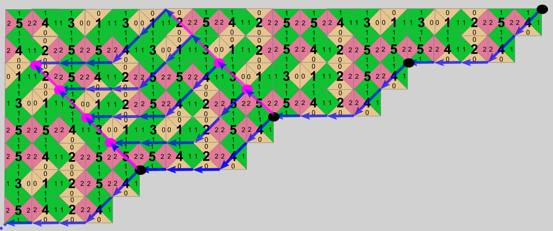
From there, consider the translation of the parity vector, one up and one right, represented between the two magenta points below (I only put one instance, not to flood the screen):
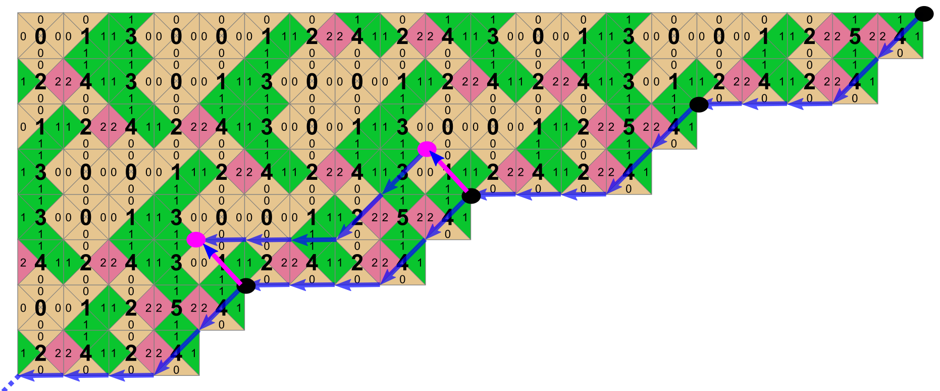
This new valued path reads:
[(↙,3), (↙,2), (←,1), (←,0), (←,0)]
Hence in our graph, we add the edge:
[(↙,4), (↙,4), (←,0), (←,0), (←,0)] ⟶ [(↙,3), (↙,2), (←,1), (←,0), (←,0)]
Furthermore, we label this arrow by (↖, 1) which is what we read under the magenta arrow in the above example. You can also add edges labelled by other translations than “one up one left”, see collapsable below. In the following, we ignore these extra edges, i.e. all our edges are labelled by ↖.
Neighbours for ←, ↑ and ↗.
We can also add additional neighbours for the translations `←`, `↑` and `↗`, which in the above case gives, in total, the edges:[(↙,4), (↙,4), (←,0), (←,0), (←,0)]⟶[(↙,3), (↙,2), (←,1), (←,0), (←,0)], labelled(↖, 1)[(↙,4), (↙,4), (←,0), (←,0), (←,0)]⟶[(↙,1), (↙,5), (←,0), (←,1), (←,0)], labelled(↑, 1)[(↙,4), (↙,4), (←,0), (←,0), (←,0)]⟶[(↙,5), (↙,2), (←,0), (←,0), (←,1)], labelled(←, 1)[(↙,4), (↙,4), (←,0), (←,0), (←,0)]⟶[(↙,2), (↙,4), (←,1), (←,0), (←,1)], labelled(↗, 2)
Using these cyclic tilings, you can make this construction for all the possible valued paths of the graph (288 in our example) and that way construct all the edges.
What’s the point?
Call 0 the valued path where all values are 0, e.g. in our case [(↙,0),(↙,0),(←,0),(←,0),(←,0)].
Then, from my thesis, we know that the parity vector creates a non-negative integer cycle if and only if the valued path obtained from the parity vector (e.g. in our example, [(↙,4), (↙,4), (←,0), (←,0), (←,0)]) and 0 (e.g. in our example, [(↙,0),(↙,0),(←,0),(←,0),(←,0)]) are in the same connected component of the graph of valued paths.
Said otherwise, it’s worth studying the connected component of 0.
For instance, here is the connected component of [(↙,0),(↙,0),(←,0),(←,0),(←,0)] (in the subgraph where we consider edges labelled by ![]() , i.e. translations by “one up one left”):
, i.e. translations by “one up one left”):
{(('↙', 0), ('↙', 0), ('←', 0), ('←', 0), ('←', 0)),
 (('↙', 0), ('↙', 1), ('←', 0), ('←', 0), ('←', 0)),
 (('↙', 0), ('↙', 2), ('←', 1), ('←', 0), ('←', 0)),
 (('↙', 1), ('↙', 0), ('←', 0), ('←', 0), ('←', 0)),
 (('↙', 1), ('↙', 1), ('←', 0), ('←', 0), ('←', 0)),
 (('↙', 1), ('↙', 2), ('←', 1), ('←', 0), ('←', 0)),
 (('↙', 2), ('↙', 3), ('←', 1), ('←', 0), ('←', 0)),
 (('↙', 2), ('↙', 4), ('←', 0), ('←', 1), ('←', 0)),
 (('↙', 2), ('↙', 5), ('←', 0), ('←', 1), ('←', 0))}
This one is cute ![]() we kind of see a numeral system. And, we clearly have that
we kind of see a numeral system. And, we clearly have that [(↙,4), (↙,4), (←,0), (←,0), (←,0)] is not in the connected component.
Function computed by valued paths in the component of 0
The function computed by any valued path of the connected component of 0 (see preamble) is the same, of the form x \mapsto Ax + 0, while in other components, the function is generally different for all the elements, e.g. the function computed by [(↙,4), (↙,4), (←,0), (←,0), (←,0)] is \frac{9}{32}x + \frac{5}{32} and the one its successor [(↙,3), (↙,2), (←,1), (←,0), (←,0)] is \frac{9}{32}x - \frac{3}{32}. And, yes, the factor in front of x is always 3^k/2^n with k the number of 1s in the parity vectors and n the length of the parity vector.
Of course, Collatz being Collatz, we can quickly encounter connected components of 0 that just look chaotic/“meh”, example in collapsable below.
Connected component of 0 for parity vector [0,1,1,1]
Here we consider parity vector [0,1,1,1], hence, 0 = [(←, 0), (↙, 0), (↙, 0), (↙, 0)]
{(('←', 0), ('↙', 0), ('↙', 0), ('↙', 0)),
 (('←', 0), ('↙', 0), ('↙', 0), ('↙', 1)),
 (('←', 0), ('↙', 0), ('↙', 1), ('↙', 0)),
 (('←', 0), ('↙', 0), ('↙', 1), ('↙', 1)),
 (('←', 0), ('↙', 1), ('↙', 0), ('↙', 0)),
 (('←', 0), ('↙', 1), ('↙', 0), ('↙', 1)),
 (('←', 0), ('↙', 1), ('↙', 1), ('↙', 0)),
 (('←', 0), ('↙', 1), ('↙', 1), ('↙', 1)),
 (('←', 0), ('↙', 3), ('↙', 3), ('↙', 4)),
 (('←', 0), ('↙', 3), ('↙', 3), ('↙', 5)),
 (('←', 1), ('↙', 0), ('↙', 0), ('↙', 2)),
 (('←', 1), ('↙', 0), ('↙', 1), ('↙', 2)),
 (('←', 1), ('↙', 0), ('↙', 2), ('↙', 3)),
 (('←', 1), ('↙', 1), ('↙', 0), ('↙', 2)),
 (('←', 1), ('↙', 1), ('↙', 1), ('↙', 2)),
 (('←', 1), ('↙', 1), ('↙', 2), ('↙', 3)),
 (('←', 1), ('↙', 2), ('↙', 3), ('↙', 3)),
 (('←', 1), ('↙', 3), ('↙', 4), ('↙', 0)),
 (('←', 1), ('↙', 3), ('↙', 4), ('↙', 1)),
 (('←', 1), ('↙', 3), ('↙', 5), ('↙', 0)),
 (('←', 1), ('↙', 3), ('↙', 5), ('↙', 1))}
Then what?
For the moment, I have studied this graph in a rather entropic way and don’t have much to say but the following two things:
First thing
The connected component of 0 always has a symmetric, which we shall call the connected component of valued path which we call -1 where all diagonal arrows have value 5 and horizontal arrows have value 1. For instance, here is the connected component of -1 = [(↙,5), (↙,5), (←,1), (←,1), (←,1)] in our previous example:
{(('↙', 3), ('↙', 0), ('←', 1), ('←', 0), ('←', 1)),
 (('↙', 3), ('↙', 1), ('←', 1), ('←', 0), ('←', 1)),
 (('↙', 3), ('↙', 2), ('←', 0), ('←', 1), ('←', 1)),
 (('↙', 4), ('↙', 3), ('←', 0), ('←', 1), ('←', 1)),
 (('↙', 4), ('↙', 4), ('←', 1), ('←', 1), ('←', 1)),
 (('↙', 4), ('↙', 5), ('←', 1), ('←', 1), ('←', 1)),
 (('↙', 5), ('↙', 3), ('←', 0), ('←', 1), ('←', 1)),
 (('↙', 5), ('↙', 4), ('←', 1), ('←', 1), ('←', 1)),
 (('↙', 5), ('↙', 5), ('←', 1), ('←', 1), ('←', 1))}
The connected components experimentally always have the same number of elements and I’m 99% sure that they are always isomorphic, in a way that is still to be characterised. Note that there is a known “multiplication by -1” operation on tilings that always work: swap all tiles 5 by 0, 2 by 3 and 1 by 4, and you get a valid tiling where each number is multiplied by -1. I strongly suspect this what is at play here.
Second thing
For each valued path, the graph has by definition the structure of a functional graph, meaning that the out-degree of each node is 1. This means that each connected component consists of a unique cycle of valued path (the attractor cycle), which I call kernel (not to confuse with Collatz cycles) and a collection of trees whose vertices eventually flow into it.
And now, something fun about kernel sizes, which is experimentally true but that I don’t understand:
Experimentally, the number of components and the distribution of kernel sizes is only a function of the number of 1s in the parity vector.
Here is this phenomenon examplified for all irreducible parity vectors of size 6: for each, I construct the graph of valued paths, count the number of components and then list the number of elements per components and per components’ kernel.
For instance, each parity vector with four 1s has 3 components and although components sizes may very, distribution of kernel sizes 1,16,1.
Also, in the below I marked the component of 0 with ° in the size columns, of the parity vector with + and of -1 with ^. You can see that in general, the component of the parity vector is way bigger than the components of 0 and -1. Also note that no component is both marked with ° and + since we don’t show (0, 1, 0, 1, 0, 1) which is three repetitions of the trivial parity vectors, as (0, 1, 0, 1, 0, 1) is not irreducible.
parity vector: (0, 0, 0, 0, 0, 1)
	components: 3
		size	kernel size
		3°	    1
		186+    60
		3^	    1

parity vector: (0, 0, 0, 0, 1, 1)
	components: 11
		size	kernel size
		9°	    1
		104	    10
		107	    10
		107	    10
		104	    10
		100+	10
		9	    1
		9	    1
		9	    1
		9	    1
		9^	    1

parity vector: (0, 0, 0, 1, 0, 1)
	components: 11
		size	kernel size
		9°	1
		106	    10
		104	    10
		104	    10
		106+    10
		98	    10
		11	    1
		9	    1
		9	    1
		11	    1
		9^	    1

parity vector: (0, 0, 0, 1, 1, 1)
	components: 11
		size	kernel size
		27°	    1
		188	    4
		194	    4
		188	    4
		190	    4
		182	    4
		188	    4
		176	    4
		182+    4
		186	    4
		27^	    1

parity vector: (0, 0, 1, 0, 1, 1)
	components: 11
		size	kernel size
		31°	    1
		190	    4
		196+    4
		210	    4
		174	    4
		182	    4
		186	    4
		212	    4
		150	    4
		166	    4
		31^	    1

parity vector: (0, 0, 1, 1, 0, 1)
	components: 11
		size	kernel size
		29°	    1
		188	    4
		192	    4
		184	    4
		170	    4
		200	    4
		194	    4
		180+	4
		184	    4
		178	    4
		29^	    1

parity vector: (0, 0, 1, 1, 1, 1)
	components: 3
		size	kernel size
		159°	1
		4866+	16
		159^	1

parity vector: (0, 1, 0, 1, 1, 1)
	components: 3
		size	kernel size
		164°	1
		4856+	16
		164^	1

parity vector: (0, 1, 1, 1, 1, 1)
	components: 3
		size	kernel size
		69°	    1
		15414+	178
		69^	    1
I’d love to prove this structural fact that kernel distributions are the same (at least, experimentally) for parity vectors with same number of 1s! This fact gives me the hope that these kernels might be… isomorphic among parity vectors with same number of 1s which could be useful in order to put these parity vectors “in the same bag”.
Summary & next steps
- Studying non-negative Collatz cycles can be reduced to studying the connected component of 0 in the graph of valued paths (and, I think, studying negative Collatz cycles can be reduced to studying the connected component of -1).
- As pointed above, this graph seems to have some valuable structure.
- The nice thing about these graphs is that it is easy to generate them and construct a big database of them (for instance, for irreducible parity vectors up to length… 20 or so).
- This data could be useful in order to, maybe, understand the connected component of 0 or at least in some cases.
Don’t hesitate to ask any question you may have ![]()