Two shortcut functions to be used with any 3n + d system

[mahfoud202]

Define:

\mathcal{J}_{1}(n, d) = \begin{cases} \dfrac{9n + d + 2}{6} & \text{if } n \equiv 1 \pmod{2} \\ \dfrac{9n + 2d - 2}{12} & \text{if } n \equiv 0 \pmod{4} \\ \dfrac{n - 2}{4} & \text{if } n \equiv 2 \pmod{4} \\ \end{cases}

\mathcal{J}_{2}(n, d) = \begin{cases} \dfrac{9n + d + 1}{6} & \text{if } n \equiv 0 \pmod{2} \\ \dfrac{9n + 2d - 1}{12} & \text{if } n \equiv 3 \pmod{4} \\ \dfrac{n - 1}{4} & \text{if } n \equiv 1 \pmod{4} \\ \end{cases}

Depending on the congruence class of d mod 6, either \mathcal{J}_{1} (for d \equiv 1 \pmod{6}) or \mathcal{J}_2 (for d \equiv 5 \pmod{6}) is used.

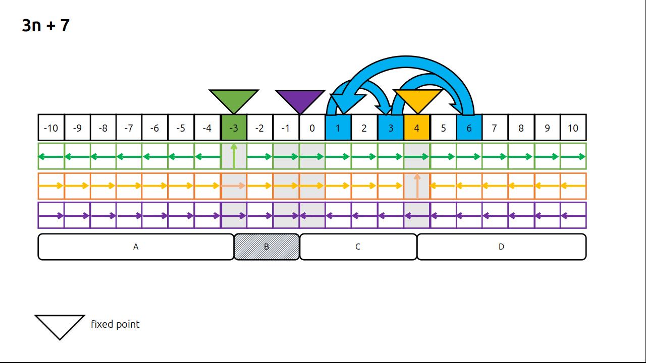
For example, the shortcut function associated with the 3n + 1 system is:

\mathcal{J}_{1}(n, 1) = \begin{cases} \dfrac{3n + 1}{2} & \text{if } n \equiv 1 \pmod{2} \\ \dfrac{3n}{4} & \text{if } n \equiv 0 \pmod{4} \\ \dfrac{n - 2}{4} & \text{if } n \equiv 2 \pmod{4} \\ \end{cases}

To demonstrate that this function is indeed a shortcut function, let us consider 17 as an example.

First, we convert 17 to its index: \dfrac{17-2}{3} = 5 (We subtract 2 when using \mathcal{J}_1 and 1 when using \mathcal{J}_2)

The trajectory of 5 under \mathcal{J}_{1} is:

5 \rightarrow 8 \rightarrow 6 \rightarrow 1 \rightarrow 2 \rightarrow 0

Multiply each value in the trajectory by 3 and add 2.

17 \rightarrow 26 \rightarrow 20 \rightarrow 5 \rightarrow 8 \rightarrow 2

Now the trajectory of 17 under Terras map defined as

T(n) = \begin{cases} \dfrac{3n + 1}{2} & \text{if } n \equiv 1 \pmod{2} \\ \dfrac{n}{2} & \text{if } n \equiv 0 \pmod{2} \\ \end{cases}

is:

\mathbf{17} \rightarrow \mathbf{26} \rightarrow 13 \rightarrow \mathbf{20} \rightarrow 10 \rightarrow \mathbf{5} \rightarrow \mathbf{8} \rightarrow 4 \rightarrow \mathbf{2} \rightarrow 1

As we can see, we hit the same values as before.

An alternative phrasing of the Collatz conjecture uses the function \mathcal{J}: \mathbb{N} \to \mathbb{N} defined by:

\mathcal{J}(n) = \begin{cases} \dfrac{3n + 1}{2} & \text{if } n \equiv 1 \pmod{2} \\ \dfrac{3n}{4} & \text{if } n \equiv 0 \pmod{4} \\ \dfrac{n - 2}{4} & \text{if } n \equiv 2 \pmod{4} \\ \end{cases}

The conjecture then states that for every n \in \mathbb{N}, repeated iteration of \mathcal{J} eventually reaches \mathbf{0}.

[mahfoud202]

A “circuit” can be defined as a sequence under \mathcal{J} that takes k steps up followed by m steps down returning to the same starting value. Since there is one way to go up but two distinct ways to go down, this leads to two types of potential circuits. Is it possible to prove that neither type can form?

[mahfoud202]

An example of a circuit loop in the 3n + 7 system using the \mathcal{J}_1 function.

[mathkook]

really cool, have to study this … so “normal 3n+5” goes 7, 13, 22, 11, 19, 31, 49, 76, 38, 19. alternately, put 7 through (n-1)/2 =2, and put 2 through the #2 function: 2, 4, 7, 6, 10, 16, 24, 6. converting these back with (3n+1) gives the shortcut trajectory 7, 13, 22, 19, 31, 49, 76, 19. what if wanted to start with 3 instead of 7 … (oh, that is probably a shortcutted-type number.)

[exstyle]

Hello,

Very interesting !!!

It seems your work echo a bit what i’m working on. As I’m a newbe in this, I hope my answer is somehow relevant and I don’t lose your time In case it’s not relevant at all, I collapsed it, to not pollute.

As my english is not that good, I corrected it wih llc helps.

**UPδ ↔ shortcut functions (3n±1): tiny cross-walk**

Your shortcut functions match the “distance-based” odd-only encoding I use for 3n\pm1.

---

UPδ packaging (per distance D)

r^-(D)=2D-1
r^+(D)=4D+1
Y_\pm(D)=3D\pm1
\mathrm{med}(D)=3D

This keeps both branches visible:

• “−” branch: r^-(D) with link Y_-(D)=3D-1.
• “+” branch: r^+(D) with link Y_+(D)=3D+1.

More info en Distance

What is the “distance” D?

In this note, the distance D indexes each odd step in the UPδ packaging.
It is defined so that the associated 5-tuple is
(r^-(D),\,Y_-(D),\,\mathrm{med}(D),\,Y_+(D),\,r^+(D)) = (2D-1,\,3D-1,\,3D,\,3D+1,\,4D+1).

Equivalently:

• “−” branch (minimal root): r^-(D)=2D-1 with odd link Y_-(D)=3D-1.
• “+” branch (minimal root): r^+(D)=4D+1 with odd link Y_+(D)=3D+1.
• The median is \mathrm{med}(D)=3D.

Recovering D from a root or a link

• From a minimal root r (i.e. t=\nu_2(3r+1)\in\{1,2\}):
  • if t=1 (branch “−”), then D=(r+1)/2;
  • if t=2 (branch “+”), then D=(r-1)/4;
  • if t\ge 3 (non-minimal): fold any r\equiv5\pmod 8 once via (3r-1)/2, then apply the rule above.
• From an oddized link Y:
  • if Y\equiv2\pmod 3 (this is Y_-), then D=(Y+1)/3;
  • if Y\equiv1\pmod 3 (this is Y_+), then D=(Y-1)/3.

Two handy checks

• On the “−” branch: Y_- - r^- = D.
• On the “+” branch: Y_+ - r^+ = -D.

Parity and valuations (baseline)

• If D is even, then \nu_2(3r^-+1)=1 and \nu_2(3r^+ +1)=2 (exact).
• If D is odd, extra twos can appear: \nu_2(3r^-+1)\ge 2 and \nu_2(3r^+ +1)\ge 3.

(Optional note.) When D is odd, r^-(D)=r^+\bigl((D-1)/2\bigr); minimality holds precisely for D\equiv1\pmod 4.

---

How many 2’s to divide out (same logic as your shortcuts)

Let \nu_2(\cdot) be the 2-adic valuation.

\nu_2(3r^-+1)=1+\nu_2(3D-1)
\nu_2(3r^++1)=2+\nu_2(3D+1)

So:

• Y^- has at least 1 division by 2 (and exactly 1 when D is even).
• Y^+ has at least 2 divisions (and exactly 2 when D is even).
• For odd D, extra divisions appear — exactly what your shortcut formulas pick by residue class.

— Sum up —

Equivalence (dictionary). For a distance D,

• r^-(D)=2D-1, r^+(D)=4D+1, Y_\pm(D)=3D\pm1.
• J₁(n,1) chooses exactly the number of 2’s to divide according to n\bmod4; in UPδ this is
  v_2(3r^-+1)=1+v_2(3D-1) and v_2(3r^++1)=2+v_2(3D+1).
  So your “one or two divisions” is the baseline (even D), with extra divisions when D is odd.
• Clean branch label: Y_-\equiv2\pmod3, Y_+\equiv1\pmod3 for all D.

Tiny lemma for your “circuits”. Let f(x)=2x-1 and g(x)=(x-1)/4 when x\equiv1\pmod4.
On distances, two “down” moves then one “up/4” always reduce D by 1:
(g\circ f^2)(D)=D-1.
So any closed circuit must compensate these -1 drifts with blocks that increase D,
which exactly corresponds to the cases where extra divisions occur (your J₁/J₂ residue cases).
This reframes your circuits as a balance of “distance drift” vs “extra divisions”.

---

Clean branch labeling (mod 3)

Because Y_- \equiv 2 \pmod{3} and Y_+ \equiv 1 \pmod{3} for all D,
the residue mod 3 identifies the branch directly (this refers to Y_\pm=3D\pm1).

---

Bridge to the 3x−1 variant

A neat identity links both worlds:

\frac{3r_+(D)-1}{2}=r_-(3D+1)

In words : folding a “+” root with the 3x-1 link lands you on a minimal “−” root at distance 3D+1.

---

Tiny examples (oddized links, 1\le D\le12)

D	r-	v2(3r-+1)	Y- (oddize)	Y- mod 3	r+	v2(3r++1)	Y+ (oddize)	Y+ mod 3	med = 3D
1	1	2	1	1	5	3	1	1	3
2	3	1	5	2	9	2	7	1	6
3	5	3	1	1	13	3	1	1	9
4	7	1	11	2	17	2	13	1	12
5	9	2	7	1	21	3	1	1	15
6	11	1	17	2	25	2	19	1	18
7	13	3	5	2	29	3	1	1	21
8	15	1	23	2	33	2	25	1	24
9	17	2	13	1	37	4	7	1	27
10	19	1	29	2	41	2	31	1	30
11	21	2	23	2	45	3	5	2	33
12	23	1	35	2	49	2	37	1	36

* Odd (D) values show extra 2-divisions beyond the base (1 / 2).
Example: D=9: 3D-1=26=2\times13\Rightarrow Y_-=13.
3r_++1=112=16\times7\Rightarrow Y_+=7.
Both stay consistent with the mod 3 rule: Y_-\equiv2, Y_+\equiv1.

Residue / structure table (regular mod 8 and mod 3 pattern)

D	r−	Y−	med	Y+	r+	r− (mod 8)	Y± (mod 3)	r+ (mod 4)	j	2+j
1	1	2	3	4	5	1	2 / 1	1	2	4
2	3	5	6	7	9	3	2 / 1	1	0	2
3	5	8	9	10	13	5	2 / 1	1	1	3
4	7	11	12	13	17	7	2 / 1	1	0	2
5	9	14	15	16	21	1	2 / 1	1	4	6
6	11	17	18	19	25	3	2 / 1	1	0	2
7	13	20	21	22	29	5	2 / 1	1	1	3
8	15	23	24	25	33	7	2 / 1	1	0	2
9	17	26	27	28	37	1	2 / 1	1	2	4
10	19	29	30	31	41	3	2 / 1	1	0	2
11	21	32	33	34	45	5	2 / 1	1	1	3
12	23	35	36	37	49	7	2 / 1	1	0	2
13	25	38	39	40	53	1	2 / 1	1	3	5
14	27	41	42	43	57	3	2 / 1	1	0	2
15	29	44	45	46	61	5	2 / 1	1	1	3
16	31	47	48	49	65	7	2 / 1	1	0	2

This “residue view” shows:

• the strict alternation of r^-\bmod8 in \{1,3,5,7\};
• Y_-\equiv2, Y_+\equiv1\pmod3 across all D;
• and the regular repetition every 4 or 8 steps of the pair (r^-,r^+).

---

Takeaway

Your shortcut operators decide how many twos to divide in one shot.
The UPδ formulation keeps both branches (Y^-,Y^+) and the distance D explicit, which helps visualize structure (sibling columns × 4, residues mod 3, and parity of valuations).

---

---

Bonus — why the rule (x-1)/4 if x\equiv1\pmod 4, else 2x-1 makes sense here

Define f(x)=(x-1)/4 if x\equiv1\pmod 4, and f(x)=2x-1 otherwise.

In our UPδ framework: r^-(D)=2D-1, r^+(D)=4D+1, Y_\pm(D)=3D\pm1, and \mathrm{med}(D)=3D.

• On a + root we always have r^+(D)\equiv1\pmod 4, hence f(r^+(D))=(r^+(D)-1)/4=D.
  In other words, f inverts the embedding D\mapsto r^+=4D+1.
• For any odd x with x\not\equiv1\pmod 4, we are in the other branch and f(x)=2x-1.
  In particular f(D)=2D-1=r^-(D) and f(r^-(D))=4D-3: we move forward linearly along the same “−” family.

What this rule establishes is a canonical normalization on the UPδ table.
Whenever we hit a + root (\equiv1\pmod 4), one application of f folds it back to its distance D; otherwise, f stays in the “−” world via 2x-1.
Equivalently, r^+(D)=4D+1\Leftrightarrow f(r^+(D))=D and r^-(D)=2D-1\Leftrightarrow f(D)=r^-(D), which justifies the mod-4 switch in this framework.

---

Bonus (addendum) — the “−, −, then +/4” reduction

Let f(x)=2x-1 (the “−” arm) and g(x)=(x-1)/4 when x\equiv1\pmod4 (the “+ then /4” arm).
Recall r^-(D)=2D-1 and r^+(D)=4D+1.

Key fact. For any odd x, we have 2x-1\equiv1\pmod4.
So one f from any odd input lands you in the 1\bmod4 class, where g is applicable.

Folding loop on distances. For any integer D:

• f(D)=2D-1=r^-(D),
• f(r^-(D))=2(2D-1)-1=4D-3=r^+(D-1),
• g\!\bigl(r^+(D-1)\bigr)=(r^+(D-1)-1)/4=D-1.

Hence the composition **always reduces the distance by 1:

(g\circ f^2)(D)=D-1.

By iteration, for any m\ge1,

(g\circ f^2)^m(D)=D-m

(as long as each step remains defined).

Example.
D=9: f(D)=17=r^-(9), then f(17)=33=r^+(8), and finally g(33)=(33-1)/4=8=D-1.

Reading in UPδ. The identity f^2(D)=r^+(D-1) shows that two consecutive “−” moves land exactly on the “+” root of the previous distance; then one g brings you back to that distance. This is the algebraic reason the mod-4 switch is the right normalizer in this framework.

Scope note. This reduction is a structural normalization on the UPδ skeleton; by itself it doesn’t prove global termination of Collatz. It’s a convenient way to fold runs of “−” steps into a shorter distance sequence.

[X0rr0]

Cool, I wanted to make the link with rational Collatz cycles with denominators of the type D = 2^k-3^x.

Here is an exchange with Chatgpt about it:

Example of a J_2 cycle

A known J_2-cycle is

8 → 12 → 18 → 27 → 20 → 30 → 45 → 11 → 8

Each branch is affine, of the form n \rightarrow a_i n + b_i, with
a,b depending on the congruence class of n:

n\mod4	rule	a	b
0,2 (even)	n\rightarrow \frac{3n}{2}	\frac{3}{2}	0
3	n\rightarrow \frac{3n-1}{4}	\frac{3}{4}	-\frac{1}{4}
1	n\rightarrow \frac{n-1}{4}	\frac{1}{4}	-\frac{1}{4}

---

Composing the 8 affine steps yields:

\Phi(n) = \frac{3^7}{2^{11}}\,n - \frac{139}{2^8} = \frac{2187}{2048}\,n - \frac{139}{256}.

A J_2-cycle is a fixed point of this composition, \Phi(n)=n:

n = \frac{2187}{2048}\,n - \frac{139}{256} \rightarrow n = \frac{-139/256}{1 - 2187/2048} = \frac{-139/256}{-139/2048} = \boxed{\,n = 8\,}.

---

This is exactly the rational-cycle condition:

n = \frac{C}{2^k - 3^x} \text{ with } x = 7,\; k = 11,\; C = -139,

since 2^{11} - 3^7 = 2048 - 2187 = -139.
But here the -139 simplifies.

---

Decoding to the real 3n-1 orbit

Decoding N=3n+1 gives:

n: 8,12,18,27,20,30,45,11 ⟼ N: 25,37,55,82,61,91,136,34

Under T_{-1} these form the periodic orbit:

25→37→55→82→61→91→136→68→34→17→25

The three interleaved numbers 68,34,17 are \equiv 2 \pmod 3,
so they are skipped by the J_2 compression, leaving the 8-node index loop above.

---

Takeaway

Any finite J_2-cycle (for 3n-1) gives a composition:

\Phi(n) = \frac{3^x\,n + C}{2^k},

and the cycle condition \Phi(n) = n yields the familiar rational equation:

n = \frac{C}{2^k - 3^x}.

Thus the J_2 functions offer a 2-adic, modular view of the same
rational-cycle denominators 2^k-3^x that appear in the algebraic analysis
of 3n-1 or 3n+1 systems.

---

[mahfoud202]

The function \mathcal{J}_1 only jumps to indices where the “normal” value is congruent to 2 modulo 3, thereby skipping all values that are congruent to 0 or 1. Conversely, \mathcal{J}_2 only jumps to indices where the value is congruent to 1 modulo 3, skipping those congruent to 0 or 2. This approach allows us to study the fundamental dynamics by focusing exclusively on these key indices and the systems’ core dynamics are still fully preserved.

[mahfoud202]

If one begins with the number 3 in this case, the two standard rules are first applied until a value congruent to 1 modulo 3 is reached. At that stage, one could perform the transformation (n−1)/3 and then apply \mathcal{J}_2.​ However, this step is not necessary. In effect, \mathcal{J}_2 performs the “tree shaking” directly, so it is possible to work solely with indices, starting from any integer.