Maximum odd-part beta difference at different LRS

Let any parity vector v have length l(v).

Call A its longest repeated substring (with wraparound), with length l(A).

We already know that vectors for which l(A) > 0.38\, l(v) are not integer cycles; if they were, the difference between the cycle members associated with AB and AC would be an integer.

\cfrac{\beta(AC)}{\delta(v)}-\cfrac{\beta(AB)}{\delta(v)} = \cfrac{2^{l(A)}\, (\beta(C)-\beta(B))}{\delta(v)}

We can cancel the 2s without affecting integrality. But then the result is not, in fact, an integer, because it’s less than one (and not zero):

\cfrac{\beta(C) - \beta(B)}{\delta(v)} < \cfrac{3^{l(v)-l(A)}}{2^{l(v)}\, l(v)^{-13.3}} < \cfrac{3^{0.62\,l(v)}}{2^{l(v)}}\, l(v)^{13.3} \ll 1

The first step above is justified by the worst case where B=1^* 0 and C=0 1^* (numerator upper bound), and by Rhin (denominator lower bound).

But what if l(A) is short, even as short as \lfloor \log l(v) \rfloor? Then we have fewer 2s to cancel, but on the other hand, the worst case B=1^* 0, C=0 1^* can’t happen, because AC (and therefore v) would have an LRS longer than l(A).

Question.

Among those v with a specified LRS of length l(A), how big can \beta(C)-\beta(B) get?

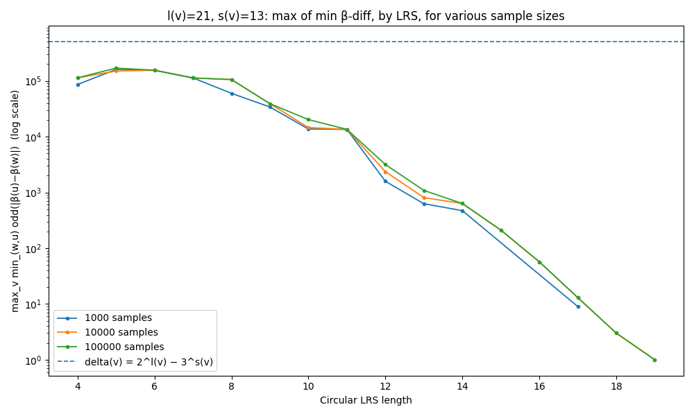
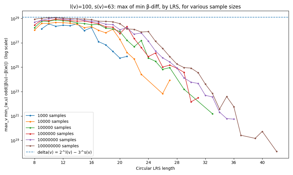
The very, very rough graph below shows the case for l(v)=100, with different values of l(A) along the x-axis.

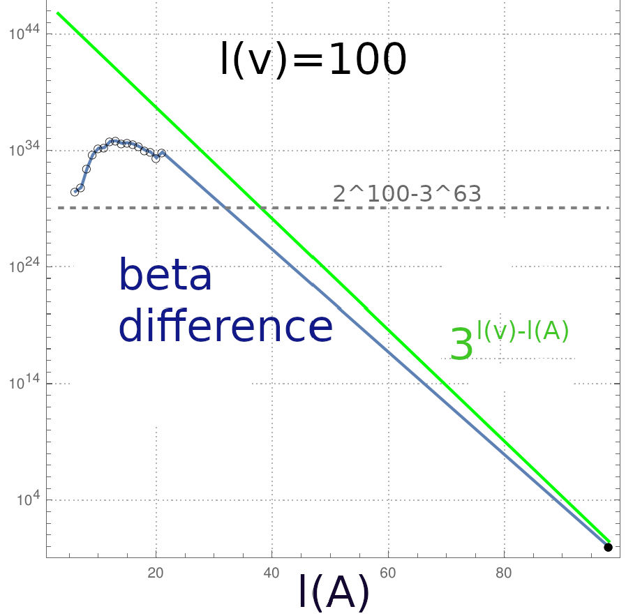
The blue line shows the (approximate) maximum possible \beta(C)-\beta(B) at each l(A). When the difference is less than \delta(v) (the dashed gray line), v is certifiably not an integer cycle. Anything above the dashed gray line is up for grabs.

The green line shows 3^{l(v)-l(A)}, a true upper bound on \beta(C)-\beta(B), but one that is very loose for small l(A).

Notice that for small l(v)=100, we cannot rule out vectors with small LRSs as integer cycles (blue line above gray dashed line). But strange things happen at small values of l(v), and we don’t know what this chart looks like asymptotically.

How high does the blue curve ever get, in terms of l(v) and l(A), for sufficiently long v?

2 Likes

You compared LRS with flatness by generating every rational cycle for a few l(v) which made me think of another question for the pile: Does β(C)−β(B) > 2^k - 3^x have a tangible cutoff for high and low flatness, or additionally, high and low number of minima?

The obvious thing about generating every rational cycle lies in A100982 - OEIS where l(v) = 19 breaks a million cycles, marking a limit for reasonable computation. l(v) = 100 is on the order of 10^{41}. Even the worst cases alone might grow exponentially. Getting an idea about what happens for sufficiently long v would require either a lot of optimization in only checking uncertain cases, different kinds of data with higher uncertainty, or going straight to pure math.

@AcidicJello More good questions. To get that rough graph for l(v)=100, I did some sampling – the real graph’s max values would look smoother (and higher, but how much higher?). The existing bound would also look tighter, after l(A) > 0.38\ l(v). Answering your first questions would be great – for now, here’s an exhaustive plot for l(v)=21.

Darker dots denote smaller \beta(C)-\beta(B). The high cycle is in the upper left; the circuit is on the far right.

1 Like

Here are a few plots of min-odd-\beta-difference by LRS length. First I sample N vectors at a given l(v), s(v). Then I bin those samples by LRS and find the most “diabolical” vector in each bin, plotting it. (“Diabolical” means it has a very high min-odd-\beta-difference.) As N increases, we’re able to better locate these diabolical vectors.

For the first plot, it’s pretty much equal to exhaustively enumerating all vectors, so the envelope is reliable. For the rest, sampling means the real envelope is higher than what you see. (For l(v)=100, a deeper searching of lowish-LRS vectors is able to locate more diabolical cases, leading to the rough inverted-U-shaped graph I posted earlier.)

But you can see the general shape that’s “taking shape.”

Notably, the current upper bound is a straight line, which doesn’t model this shape well.

As usual, the main idea is that any vector below the dashed line can be ruled out as an integer Collatz cycle.

I can’t believe I forgot about sampling. I don’t want to overwhelm you with questions but I have a lot, so feel free to address as much or little as you have answers to at hand since I’ll try to answer them myself otherwise.

Does the first plot suggest to you that most or all of the short vectors where a second cycle could have been expected had a minimum odd beta difference smaller than the denominator? On the other end, do you have any level of confidence yet about whether or not the proportion of arbitrarily large vectors ruled out this way (with the 0.38 l(v) bound) is “almost none”?

By odd beta difference, do you mean the odd part of the beta difference of the original two rotations? The LRS can begin with an even step, right?

For a vector to be diabolical, it has to have a high minimum odd difference compared to the other vectors of the same size. So the minimum odd difference doesn’t always occur between the rotations with the LRS prefix? Is it a combination between the untrimmed beta values being close together (i.e. the corresponding rational cycle members are close in size) and also the overlap in prefix at those two points? Edit: I just re-read and saw you categorize them as diabolical after binning them by LRS.

What do you mean by modeling the shape? And how could it be something other than a straight line (how could it be a function of LRS length)?

Already at l(v)=27, there are vectors that can’t be ruled out by the “difference method”. This might be expected if only because \delta can be unreasonably small for short vectors, eg, 2^8-3^5=13. Or you could say, no method can rule out the trivial cycle 1-2-1 :slight_smile:

The proportion of vectors definitively ruled out by the 0.38\ l(v) bound is “almost none”.

By odd-\beta-difference, I mean \beta(w) - \beta(u) with the 2s divided out. By min-odd-\beta-difference – which we might call mobd(v) – I mean, take v and find the rotations w and u that have minimal odd-\beta-difference.

To find LRS of v, find rotations w and u with the longest shared prefix.

The two concepts are related, as you notice … with a high LRS, you expect a lower mobd. But there are plenty of exceptions.

What makes a v diabolical, though, is that none of its rotation pairs seem to “cash in” with a nice, low odd-\beta-difference. Within any LRS bin (or in general), some vectors are more diabolical than others.

We’d like an analytic upper bound on the entire curve. The straight line is way too loose on the left part of the graph. To put it another way, given some l(v) and s(v), how high is the highest point on the curve?

PS. There are complex, efficient algorithms for finding |LRS|, given v. I don’t know of an efficient algorithm for finding mobd(v), but would like one.

Oh I thought you meant the line 2^{l(v)}-3^{s(v)} but yes I understand now for the line 3^{l(v)-l(A)}

1 Like